Taming the flowsnake and visualizing Covid proteins
The Gosper curve is a well-known space-filling curve.
It sports a dual form called a flowsnake which sequentially visits
every hexagon of an infinite lattice with no jumps or crossovers,
reminiscent of the Hilbert curve on the Cartesian (square) grid.
Counting along the curve is a little slippery (it is a snake after all!)
but we’ll show how counting in negative base 7 with an
unbalanced set of signed digits (=, -, 0, 1, 2, 3, 4)
makes it easy to convert back and forth between arbitrary points along the flowsnake
and corresponding hexagons.
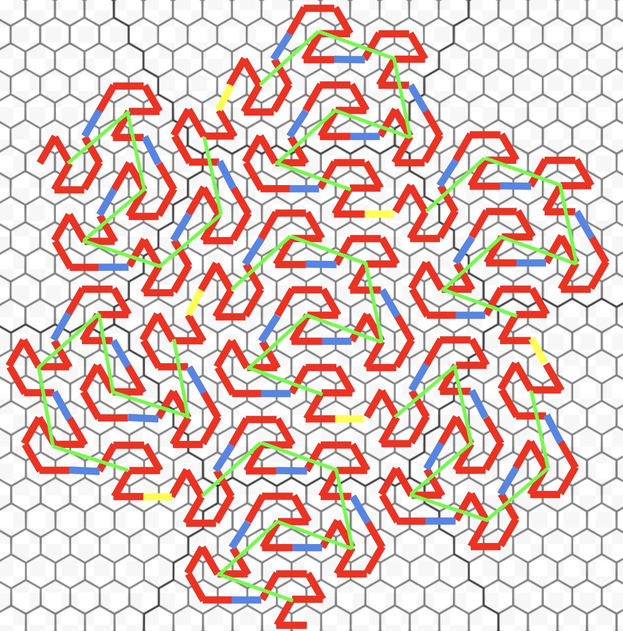
This enumeration is useful for compact visualization of one-dimensional sequence data as well as indexing and compression of hexagonal data structures with good locality properties. One example is this simple visualization of the structural protein sequence for SARS-CoV-2:
A flowsnake visualization of the structural protein of Covid-19. The amino acid sequence is centered around the origin, with individual amino acids strung along the grey flowsnake path as colored beads, based on a standard color palette. The embedding induces a specific boundary shape based on the sequence length and initial offset, with a compact “folding” reminiscent of (but of course completely unrelated to) protein folding, which perhaps provides a useful visual fingerprint for the sequence.
I stumbled on this idea via a note in Amit Patel’s great hexagonal grid reference. He links a stackoverflow question about spiral honeycomb mosaic (SHM) coordinates. This is a system for enumerating an infinite hex grid. (See also the similar generalized balanced ternary address labeling.) We count in base 7 starting with the origin at 0, and label its six immediate neighbors 1 through 6 to form a super-hex of seven individual hexagons. We repeat the process to enumerate the six neighboring super-hexes as the (base 7) tens, twenties and on through sixties to form a super-super-hex of 7*7 = 49 individual hexagons, and continue recursively (to infinity and beyond!). In the posted solutions, Patel offers a nice approach for calculating the index along the path for an arbitrary hexagon which we’ll piggyback on.
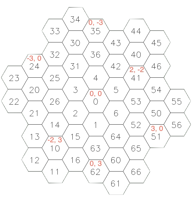
Spiral honeycomb mosaic (SHM) coordinates give a recursive enumeration of an infinite grid in base 7 (black numbers). Patel’s mapping to hexagon axial coordinates is shown with red digits.
The SHM enumeration of the hex grid is straightforward, but if we draw the path connecting sequential numbers it gets a little tangled (below). I wondered if there was a more compact approach where the path had few (or no) crossovers, so that hexes with similar indices on the path tended to be closer together. There are a bunch of examples of such space-filling curves on the normal Cartesian lattice including the Hilbert curve which is a more compact version of the more common z-order curve.
The path connects hexes ordered by SHM coordinate starting at the origin. As we see by the path and the rainbow color map over path offset, we see tangling and jumps as we connect larger and larger hex modules. The dotted red lines show how the unit vectors twist as the super-hex size grows through $1, 7, 7^2, …$.
While exploring Cartesian analogs, I came across the Gosper curve. It has a hexagonal vibe but the repeating seven segment unit doesn’t immediately look like it maps nicely to a super-hex.
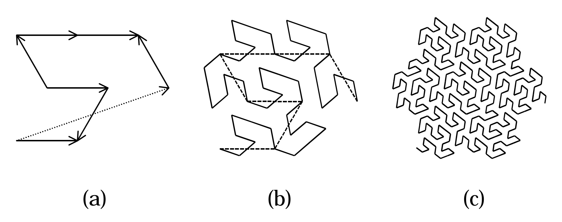
The Gosper curve is formed by a recurring motif of seven directed line segments (source).
But it turns out there’s a dual of the curve where each directed segment can be associated with a hexagon to give the flowsnake:
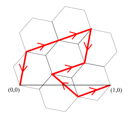
The flowsnake is a dual view of the Gosper curve formed by associating each directed segment with a hexagon, yielding a recurring 2-shaped motif of seven hexagons (source).
Linking this motif following the same pattern, we can recursively form a self-similar motif of hexes, super-hexes, super-super-hexes and so on. Here’s a hand-drawn sketch I put together to get to grips with the recurrence:
We can recursively trace a path through super-hex groupings of a central hex and their six neighbors. The seven hex motif is traced by red segments, with seven of these super-hexes connected by blue segments to form a self-similar super-super-hex motif sketched in green. Seven of these are connected with yellow segments to form another self-similar grouping and so on forever. Note how the traversal direction through the motif flips at each level.
It seems obvious that we should be able to enumerate the points on the flowsnake
in a one-to-one correspondence to the SHM enumeration but how exactly?
The SHM labeling starts at the origin and extends outwards towards infinity,
but the flowsnake motif is double-ended.
If we naively start labeling in base 7 from one end of the repeating motif (below left),
then at each recursive step the zero point gets further and further from the origin.
The solution is to use a signed digit representation
where we count from -2 through 4 in base 7, leaving 0 at the center (below right).
For convenience
we’ll write -2 as the = character (two minuses) and -1 as - (one minus).
Aside: if you want a little practice with this type of representation,
check out this puzzle from last year’s Advent of Code.

Counting with a signed representation lets us keep the origin pinned at the middle of the recurring motif. Using a negative base lets us cope with the change of direction with each level of recursion.
Unfortunately this still doesn’t quite work,
since at each recursive step we traverse the seven hex motif
in the opposite direction.
At one level we want to count like -2, -1, 0, … 4 and at the next like
-4, -3, … 0, 1, 2.
In fact with the naive base 7 enumeration, the origin would end up at 2424242... and recede off toward infinity.
One last trick gets us there: let’s count in negative base seven!
What?! Starting from 0 we’ll count like 0, 1, 2, 3, 4, 1=, 1- 10, 11, ...
where a number like =21 means $(-2)(-7)^2 + 2(-7) + 1 = -111$.
Conversely, for any integer we find its negative base 7 representation
by casting out remainders of 7 and flipping sign at each step.
For example $125 \pmod 7 \equiv 6 \equiv -1$ so the ones digit is -
with $125 - (-1) = -18 \times -7$ left over.
Then $-18 \pmod 7 \equiv 3$ with $-18 - 3 = 3 \times -7$ left over.
This gives the representation 33-
which we read as 3 forty-nines plus 3 negative sevens plus a minus one
and indeed $3 (-7)^2 + 3 (-7) + (-1) = 125$.
Phew!
1
2
3
4
5
6
7
8
9
10
11
12
 -idx       g7       shm         axial hex
----------------------------------------------
   -3        14        24     {q:   1, r:  1}
   -2         =         2     {q:   0, r:  1}
   -1         -         3     {q:  -1, r:  1}
    0         0         0     {q:   0, r:  0}
    1         1         1     {q:   1, r:  0}
    2         2         6     {q:   1, r: -1}
    3         3         5     {q:   0, r: -1}
   10        -3        43     {q:  -4, r:  3}
  100       202       216     {q:  12, r: -6}
 1000     1404-     51011     {q: -13, r: 35}
A few examples illustrating conversion from an index value idx to the corresponding
g7, shm and axial hex coordinate.
Note we flip the idx sign so that 0 and 1 are common in all three systems.
The g7 value ranges over all positive and negative integers written as digits =-01234,
shm is a non-negative integer written in base 7 with digits 0123456,
and the axial hex coordinate uses Patel’s cubical system.
Now we have all the ingredients to tame the flowsnake.
If you want the gory details here’s the enumeration code,
but the end result is surprisingly simple (ignoring the painful journey there).
We can convert back and forth from an integer to its g7 (Gosper7) representation
with inttog7 and g7toint.
Converting between g7 and SHM numbering is easy via g7toshm and shmtog7
and once we have a SHM coordinate we can find axial hex coordinates or vice versa
with shmtohex and hextoshm, all in $\mathcal{O}(\log_7 n)$ steps.
Once we can go back and forth between arbitrary flowsnake indices and hexagon locations
we’re ready to experiment with data visualization and indexing or compressing
hexagonally structured data.
Our flowsnake path connects hexes ordered by their G7 coordinate.
The origin is pinned at 0 with the path extending in both directions from there.
All the tangling and jumps from the SHM path have been removed,
and the color map over path index shows much nicer locality properties.
More food for thought
My initial motivation was simple curiosity and a vague idea of an efficient one-dimensional enumeration of the infinite hexagonal grid forming a universal identifier for hex maps. Although it’s an elegant solution I’m not sure it’s worth the effort in practice. But as we know hexagons are the bestagons so a number of other ideas popped up as I struggled to make the enumeration code work:
- Can we quantify “nice locality properties”? It seems obvious that the flowsnake enumeration is better at assigning nearby hexes similar index values than SHM or a simple spiral enumeration from the origin, but it would be interesting to measure that. One approach seems to be choosing random compact hexagon regions and measuring the correlation between region size and index variance or number of index skips within the region. For example see Analysis of the Clustering Properties of the Hilbert Space-Filling Curve.
- Are there alternative flowsnake enumerations or different space-filling curves on hexagons? Kevin Ryde offers an interesting three-armed construction and enumeration of a flowsnake-like curve in his intriguing planepath package.
- I also wondered: is there a Cartesian analogue of the flowsnake?. Spoiler alert, yes. I’ll make a quick post about that soon.
- I don’t really know anything about DNA sequence analysis or visualization. Is something like the Covid19 example above actually useful? There’s a good survey of techniques in Tasks, Techniques, and Tools for Genomic Data Visualization including work on High resolution visualization of genomic data with Hilbert curve which looks like it suffers from binary grid artifacts that might be ameliorated by a hexagonal grid.
- Are there other interesting sequential data visualization use cases? The canonical example is Mapping the entire internet with Hilbert curves but that actually seems to benefit from a binary segmentation given how IP addresses are constructed. Visualization of rransformer models and recurrent neural networks might be interesting to explore.
- Could we use recursive hexagonal partitioning as an alternative to traditional geohashing code which uses a z-order curve on latitude and longitude? The direct latitude/longitude projection means geohash squares are far from equal area as latitude changes. Could we use a geographic projection that results in roughly hexagonal shape like the equal-area Eckert II projection and recursively subdivide with the flowsnake? There might be challenges with the recursive twisting of the tessellation, and the fact it doesn’t generate a pure hexagon shape, but perhaps we could wrap the edges somehow to complete the sphere? See also Uber’s H3 system representing the earth as a spherical polyhedron tiled with hexagons and a handful of strategically placed pentagons, and Google’s S2 projection of the globe onto a cube of six connected Hilbert-curves.